
In this section, there are a number of examples. The examples go from easy to more sophisticated. Here is a list of the examples and a short description of what you can expect to learn from each of the examples. You can find these examples (and more) in the examples, which is part of the PsyToolkit downloadable software package (see download section).
TIP:
All examples come with the PsyToolkit package. They are in /usr/share/doc/psytoolkit/1.9.4/examples. More examples can be found in the lessons section.
All examples come with the PsyToolkit package. They are in /usr/share/doc/psytoolkit/1.9.4/examples. More examples can be found in the lessons section.
- A simple example. Teaches you:
- How to write a script using an editor
- How to draw a stimulus using Inkscape
- How to compile a script
- How to run an experiment
- How to do some really simple statistics using R
- A Simon task. Teaches you:
- How to set up a simple choice reaction time task
- How to use rectangles as stimuli
- How to save data into a data file
- How to analyze your data with R
- An example of Inhibition of Return. Teaches you:
- How to set up a choice reaction time experiment with multiple stimuli in one trial
- A more advanced example of Inhibition of Return. Teaches you:
- How to use R for creating feedback for participants
- A example of task switching. Teaches you:
- How to use multiple tasks
- An example of using the mouse as a response devices. Teaches you:
- How to use the mouse in scripts
- How to ask the participant to click on certain areas (stimuli) of the screen
- How to use fonts
- An implementation example of the Wisconsin Card Sorting Test. Teaches you:
- How to identify which bitmaps a participant clicked
- Set and use a custom variable
- Run a fixed sequence of trials
- How to use the pager function to show multiple instruction screens
- Play sounds
- An implementation example of an attentional blink task. Teaches you:
- How to run experiments with or without a table
- How to clear multiple stimuli in one line
- An implementation example of a multiple object tracking task task. Teaches you:
- How to use moving stimuli sprites
- How to click moving stimuli with the mouse
- How to show a background image
TIP:
These examples can all be found in the downloadable PsyToolkit package!
These examples can all be found in the downloadable PsyToolkit package!
A complete guide for a simple experiment
Before we start with anything advanced, I would like to take you through a complete example of a simple experiment. It may help to get used to the idea of PsyToolkit, whilst leaving out more advanced features. I will also show how to analyze the data with the free statistical software R. This is just to give you a start and a feel for the whole approach of PsyToolkit. If you got that, you can move to the other examples further down on this page.Step 1: Design
The experiment will have 10 trials of a simple task. The task is: As soon as a red circle appears, the participant must press the space bar. After this button press, the circle appears, and will appear soon after for a next trial. The maximum allowed response time is 1 second.Step 2: Create a new directory
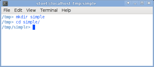
It is a good idea to create a separate directory (or "folder") for each experiment. In Linux, you can create directories either on the Command Linux Interface, or using the graphical file manager. Here, I will explain the command-line way (because you can figure the point-and-click way yourself).- Open a 'terminal window'. You can do this, on many Linux systems as follows: Go to "applications", "accessories", "terminal".
- Create a directory called simple, type mkdir simple.
- Go to this directory typing cd simple.
TIP:
Typing things into the terminal is known as a command line interface. Read more about this for Linux in this guide.
Typing things into the terminal is known as a command line interface. Read more about this for Linux in this guide.
Step 3: Create a stimulus
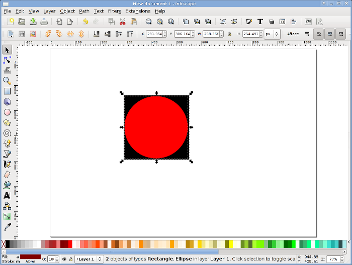
For this experiment, we need only one stimulus, a red circle. Create a red circle on a black rectangle. This way, on the black screen (the default color in PsyToolkit), you will just see a red circle.- Open Inkscape, either from the menu or by typing Inkscape on the command line.
- Draw a stimulus, for this experiment is does not really matter what it looks like. For example, click on the circle box in the left toolbox column and then draw a circle. You can fill it in a different way by clicking the right mouse button on the drawn circle and select fill and stroke. The Inkscape user interface is intuitive. When you are done with drawing the stimulus, select it by clicking on it or drawing a selection box around it.
- In Inkscape, select from the File menu the export bitmap option. You will see a dialog window. Name the bitmap mystimulus.png and click the export button (make sure you choose the right directory as well, and set the width not too big, for example 150 by 150 pixels). Now there should be a bitmap file in png format in your directory!
- Exit the Inkscape program now (but you might save the SVG file as well, the graphics file format of Inkscape, even though PsyToolkit does not use SVG files itself).
- Check whether your new file mystimulus.png exists in the correct directory. Just type ls in the terminal window to get a list of all your files in the current directory. If it does not exist, you did something wrong, and need to try Inkscape again.
You are done with the stimulus creation. If you want to learn more of how to use Inkscape, there is a good online book on how to use it: tutorial.
TIP:
Stimuli can be transparent (but that is not the default option). With transparency, you do not need to put stimuli on a black background (as in the above example). All you need to do is choose the transparency option: transparency on. A good example is the first image in the multiple object tracking task, where the faces are semi transparent (you can see the clouds through them).
Stimuli can be transparent (but that is not the default option). With transparency, you do not need to put stimuli on a black background (as in the above example). All you need to do is choose the transparency option: transparency on. A good example is the first image in the multiple object tracking task, where the faces are semi transparent (you can see the clouds through them).
Step 4: Open up an editor and write a simple script
Now you need to write your PsyToolkit script file. All this file is, is some text. You can create such a file with a text editor. Maybe you already have a favorite text editor. If not, and if you are not very familiar with text editors, you can use gedit, which is a sophisticated text editor installed on many Linux systems. Often you can select this from your desktop menu: Applications->Accessories->Text Editor. Or simply type gedit on the command line.Open editor and copy and paste this code
bitmaps
  mystimulus

task simpletask
  keys space
  delay 100
  show bitmap mystimulus
  readkey 1 1000
  clear 1
  save STATUS RT

block firstblock
  tasklist
   simpletask 10
  end
Now the same, but with full explanation of each line
                         # everything following "#" is comment
bitmaps                  # indicates definition of bitmaps
  mystimulus             # refers to the file mystimulus.png
                         # empty line means end of (bitmaps) section

task simpletask          # task indicates definition of the "simpletask"
  keys space             # there is only one key used, the space bar
  delay 100              # wait for 100 milliseconds
  show bitmap mystimulus # show the bitmap. Without XY coordinates show at center
  readkey 1 1000         # wait up to 1000 milliseconds for key number 1
  clear 1                # once key pressed (or 1000 ms passed), clear first presented stimulus
  save STATUS RT         # save the status (correct/timeout) and reaction time to file

block firstblock         # blocks tell how to run trials
  tasklist               # lists which tasks to choose from
   simpletask 10         # run simpletask 10 times
  end                    # end of task list
In gedit, it will look like this:
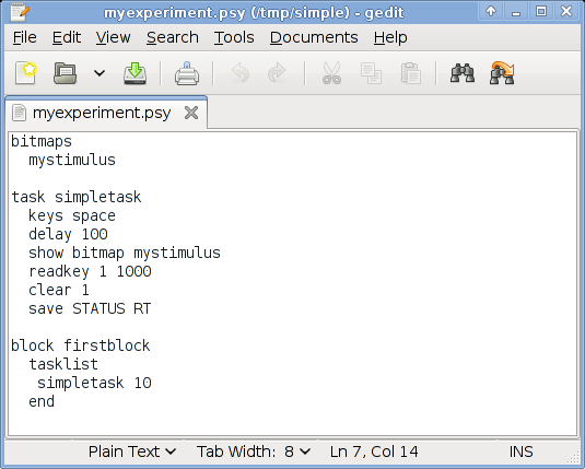
Copy and paste this in your editor. Save the file as myexperiment.psy. Make sure you save it in the right directory (that is the one you created before)! You can close the text editor, or leave it open, as you like.
As you can conclude from the example, the code consists of three parts, one describes the stimuli, one describes the task, and one describes the experimental block. Of course, you can have multiple tasks and blocks, etc, but here I just want to give a possibly simple example.
Step 5: Compile the script
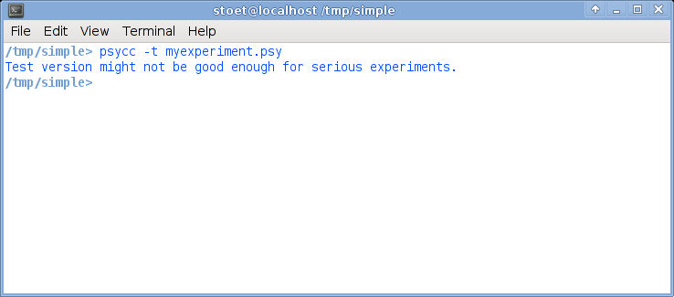
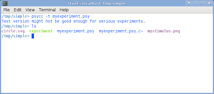
Now select your terminal window again. Now type psycc -t myexperiment.psy, obviously followed by return. The -t option tells the compiler that you just want to test, and it will run in a window, not in full screen mode.This is what it could look like:
Just for testing: List the contents of the directory (type ls to get a listing of all files in the directory). There should now be a file called experiment.
This is what it could look like:
Step 6: Test the experiment
On the command line type experiment. Nothing happens? Than the current path is probably not in your path variable. Try ./experiment, that should work for sure. You should now get a full screen experiment with 10 trials. If you see the dot, just press the space bar.This is what it could look like:
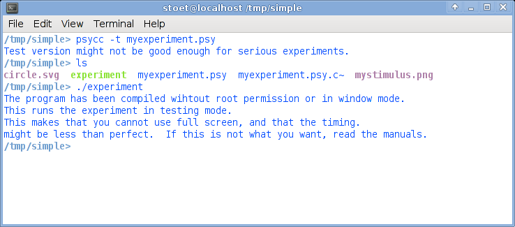
With the option -t, psycc runs in a testmode. If you want to run in regular mode, you will not get all of the messages you see now. But, because we are testing here, it is good to work in test mode. Also, when you run in testmode, you will not run in full screen mode.
TIP:
Compile with the -t option to test scripts. Once it works, you compile without -t to run in full screen mode.
Compile with the -t option to test scripts. Once it works, you compile without -t to run in full screen mode.
Step 7: Analyze the data
Now you are done and a new file should have been created, something starting with myexperiment and ending with data. Just type ls to find the new file, and type cat plus data filename to see the content (you can also see and edit the content with gedit, of course).This is what it could look like:
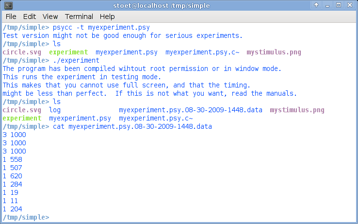
As you can see, the data file contains the date (you can open it with the text editor, it is a simple text file, with one line for each trial). Write down the file name on a piece of paper.
The first column is the status (1=correct, 3=timeout), and the second column is the time in ms. If you would never have pressed the button, all lines would have been "3 1000". For this example, I did not press the first 3 trials. Of course, you can set the maximum RT from 1000 ms to something longer.
Now type R (assuming you have installed the package R). You will get a prompt. Type the following, but replace the "DATAFILE" with the filename you just wrote down. You will get the mean response time!
data = read.table("DATAFILE")
meanrt = mean( data[ data[,1]==1 ,2] )
cat("Mean response time in correct trials is:", meanrt,"\n")
q()
That was the simple example!
More advanced examples
Before you move on, please note that the example files are located in /usr/share/psytoolkit/examples/You can only compile an example if you first copy it to a write permissible location. For example, if you want to test the simple experiment yourself, and if you are in your home directory, you can type this:
Compile and run an example experiment.
# Type the following on the command line, assuming the $ sign
# is your command line prompt:

$ cp -r /usr/share/psytoolkit/exampels/simple ./
$ cd simple
$ psycc -t -k simple.psy
$ ./experiment
Simon task, also known as spatial compatibility task
In short, compatibility tasks study the ease of difficulty of the relationship between stimuli and responses, stimuli and stimuli, or responses and responses. Examples of incompatible relationships are:- Drawing a circle with your left hand whilst drawing a rectangle with your right hand
- Responding with your left hand to something happening right of you.
Some of the early work on compatibility was done by J.R. Simon.
In the spatial compatibility task of the example, you must respond to red and green stimuli with the left shift or right shift key, respectively. If the red stimulus appears on the left side of the screen, it is easier to respond to than when it appears on the ride side of the screen.
In this example, no bitmaps are used. The aim of the example is to show how you can create simple stimuli using rectangles.
Another aim is to show positioning of stimuli. Each stimulus has an X and a Y coordinate. If you use the option centerzero, XY coordinates 0,0 refer to the screen center. Thus, if you present a stimulus at XY position -200 0 , the stimulus will be horizontally left of the screen center, and vertically in the middle. In the simon task, we present the fixation point at screen center (0,0), and the target stimuli left or right of the center.
Compile this experiment just with psycc -t simon.psy. Run the experiment by typing ./experiment. After the experiment, type ls -rtl in your terminal window, and see that some new files have been created. One of these files ends with the extension data. Open this file with a text editor. Each row of this file has the data of one trial. Each row is created by the save line of the script.
# File: examples/simon-spatial-compatibility/simon.psy

# simple Simon stimulus-response compatibility task
# instruction for participant:
#   press left shift button in response to red stimulus
#   press right shift button in response to green stimulus

options
  centerzero  # postion 0,0 is center of screen
  window      # use a window (remove this to have full screen)
  escape      # experiment can be interupter by holding escape until end of trial

table simontasktable # table with four rows, each trial one row is randomly chosen
#-name of condition--------------position--red?--green?--correct key--------------
  "leftresponse  compatible"     -200      255   0       1
  "leftresponse  incompatible"    200      255   0       1
  "rightresponse compatible"      200        0   255     2
  "rightresponse incompatible"   -200        0   255     2

task simon
  table simontasktable                   # table to be used
  keys lshift rshift                     # keys to be used
  show rectangle 0 0 10 10 255 255 255   # small white rectangle at
  delay 200                              # center for 200 ms
  clear 1                                # erase the rectangle
  delay 50                               # and wait 50 ms
  show rectangle @2 0 100 100 @3 @4 0    # target stimulus is presented
  readkey @5 5000                        # wait for key of column 5 of table
  clear 2                                # remove target stimulus from screen
  if STATUS != CORRECT
    show rectangle 0 0 10 10 255 255 255
    delay 100
    show rectangle 0 0 20 20 255 255   0
    delay 100
    show rectangle 0 0 30 50 255 255 255
    delay 100
    show rectangle 0 0 50 50 255 255   0
    delay 100
    clear 3 4 5 6
  fi
  delay 100                              # wait 100ms (here sort of intertrial time)
  save BLOCKNAME @1 TABLEROW KEY STATUS RT  # save data to file

block test    # this block is called "test"
  tasklist
    simon 40  # run the simon task 40 trials.
  end
Run the experiment and analyze the data with the following R file. Here is how you can do that:
- Run gedit from command line with gedit, and copy and paste the code below.
- Replace the filename on the read.table line with your data filename.
- Save file as analyze.r and exit gedit.
- Run R, just type R on the command line.
- On the R prompt, type source "analyze.r".
- You should now see a box plot.
# File: examples/simon-spatial-compatibility/analyze.r

# read the table. Filename has date of finishing time in it, so
# it will be different on your computer. Look up which file it is using
# ls simon*data
# on the command line.
data = read.table( "example.data" )

# boolean, True if trial was correct
correct = data[,6]==1

# boolean. True if compatible trial
compatible = data[,3]=="compatible"

# boolean. True if response was on the left
left = data[,2]=="leftresponse"

# rt is in column 7, that is data[,7]
# use cbind to combine the data vectors of the four conditions

boxplot( cbind( data[ correct &  compatible &  left, 7],
                data[ correct &  compatible & !left, 7],
                data[ correct & !compatible &  left, 7],
                data[ correct & !compatible & !left, 7]),
         names=c("left/comp","right/comp","left/incomp","right/incomp"),
         ylab="RT (ms)",col=c(3,3,2,2))
title("Box plots of RTs in the four conditions")
It might not be the case that you were slower in the incompatible trials (in red). Stimulus-response time compatibility effects can be small. You could change the number of trials to something like 500, and do the analysis again.
Inhibition Of Return
Inhibition Of Return is the phenomenon that people respond slower to a stimulus which occurs at the same position as a target. The phenomenon was first described by Michael Posner.In the following experiment, we have the following sequence of events:
- Two yellow frames, left and right of a fixation cross are simultaneously presented
- One of the two frames flashes. This should attract the attention to either the left of the right. This is called the IOR Cue.
- About a second later, within one of the two frames, a white dot appears (i.e., the IOR target), which requires an immediate left or right button press (left or right shift button)
Code: Creating a simple IOR experiment
# File: examples/ior/ior.psy

# example script doing an inhibition of return experiment
# everything following a hash mark is a comment and is ignored
# by the script interpreter

options
 window
 origin topleft
 escape     # you can escape the program
 render doublebuffer

bitmaps     # define some bitmap names, different ways to do this.
 frame        bitmaps/frame.png
 plus         bitmaps/plus.png
 dot          bitmaps/dot.png
 instruction  bitmaps/instruction.png

table standard    # table with 5 columns, which can be address with @-sign
#1                             #2 #3  #4   #5
#--------------------------------------------
 "cueleft  targetleft  cued"   2  200 200  1
 "cueleft  targetright uncued" 2  200 600  2
 "cueright targetleft  uncued" 3  600 200  1
 "cueright targetright cued"   3  600 600  2

task ior
 table standard               # use this table for choosing conditions
 keys lshift rshift           # use 2 shift keys in this experiment
 draw off                     # hold off drawing
 show bitmap plus             # 1
 show bitmap frame 200 300    # 2
 show bitmap frame 600 300    # 3
 draw on                      # now draw all three items
 delay 1500                   # wait 1500 ms
 clear @2                     # IOR cue; frame OFF attract attention
 delay 100                    # wait 100 ms
 show bitmap frame @3 300     # 4 ; frame ON again, still attacts attention
 delay 860                    # wait 860 ms
 show bitmap dot @4 300       # 5 ; show IOR target
 readkey @5 1500              # wait max 1500 ms until correct key is pressed
 clear 5                      # remove target from screen
 save BLOCKNAME @1 STATUS RT  # save trial information

message instruction           # shows instruction and waits for key press

block mainblock               # there is just one block
 tasklist
  ior 10                      # choose the ior task 100 times
 end
Note that I like indentations. They are only used for readability, they have no meaning to the interpreter. On the other hand, EMPTY LINES play a syntactical role. An empty line ends a section, such as the sections 'options', 'bitmaps', 'table', 'task', and 'block'.
Make a directory and put this code in a textfile (or go to the corresponding examples directory in the downloaded package). Get this code running by typing the following on the command line. The "$linux" part is assuming to be the prompt, this will likely be different on each system.
Compile and run
$linux> psycc ior.psy
password: your password, make sure you are in the sudo group
$linux> ./experiment
The options part has the option window. Take it out to get the default full screen mode!
Compile and run, method 2
$linux> psycc ior.psy
$linux> experiment
Now do the experiment. The data will be written to a file starting with the name of the script, and ending in data. Every data file will be unique, since it contains the date and time of the time it gets written (at the end of the data collection).
Of course, you want to analyze the data. You can do it with whatever program you like, the data is save in just plain ASCII. Here are some examples of how you can do it in R. Of course, R is a whole language on itself, and you can find great tutorials on the internet (see the resources section).
R Example: Analyze the data of a single subject
# File: examples/ior/ior-single-subject.r

files = dir(pattern="^ior\.psy.*data$")
if ( length(files) > 1 )
  {
    cat("there is more than one datafile, I will look at the first one\n")
  }
data = read.table( files[1] )
colnames(data)=c("block","cuepos","targetpos","condition","status","rt")
rt = data[,"rt"]
correct = data[,"status"]==1
cued = data[,"condition"]=="cued"
cat("Cued mean: ",
    mean(rt[correct & cued]),"\n",
    "Uncued mean: ",
    mean(rt[correct & !cued]),"\n",sep="")
R Example: Analyze the data of a group of subjects with paired Student's t tests
# File: examples/ior/ior-group.r

# assume all files ending in .data are from this experiment!
cued.all=numeric(0)
uncued.all=numeric(0)
datafiles=dir(pattern="data$")
cat("Number of subjects: ",length(datafiles),"\n")
if ( length(datafiles) < 2 ){cat("not enough data!\n")}else{
for ( i in datafiles )
  {
        x=read.table(i)
        cued = mean(x[x[,4]=="cued" & x[,5]==1,6])
        uncued = mean(x[x[,4]=="uncued" & x[,5]==1,6])
        cued.all = append( cued.all, cued )
        uncued.all = append( uncued.all, uncued )
  }
cat("Cued mean: ",mean(cued.all),"\n","Uncued mean: ",
    mean(uncued.all),"\n",sep="")
print(t.test(cued.all,uncued.all,paired=T))
}
Inhibition Of Return, but fancier.
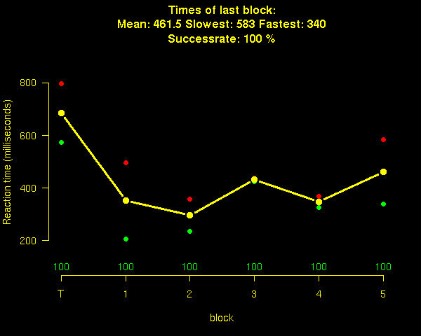
Probably you want some things look a little nicer. For example, you might want one training block, and you want blocks with pauses between them, and you would like your subjects to be motivated, so you might want to give them some feedback about their performance. The following example has all those features. Note that you can ask a block to repeat itself by adding a number in the block line. Also not that you can make a system call to access the data. In this case, following every block, we call R to analyze the data of the block and then display the results.The feedback screen looks like this:
code: ior fancy version
# File: examples/ior/ior2.psy

# example script doing an inhibition of return experiment
# everything following a hash mark is a comment and is ignored
# by the script interpreter

options
 window     # remove this if you want to run full screen
 escape     # you can escape the program
 bitmapdir  bitmaps # directory where to find bitmaps
 origin topleft

bitmaps      # define some bitmap names
 frame       # if bitmaps have png extension, you do not need to specify
 plus        # the whole file name.
 dot
 instruction

table standard    # table with 5 columns, which can be address with @-sign
#1                             #2 #3  #4   #5
#--------------------------------------------
 "cueleft  targetleft  cued"   2  200 200  1
 "cueleft  targetright uncued" 2  200 600  2
 "cueright targetleft  uncued" 3  600 200  1
 "cueright targetright cued"   3  600 600  2

task ior
 table standard               # use this table for choosing conditions
 keys lshift rshift           # use 2 shift keys in this experiment
 draw off                     # hold off drawing
 show bitmap plus             # 1
 show bitmap frame 200 300    # 2
 show bitmap frame 600 300    # 3
 draw on                      # now draw all three items
 delay 1500                   # wait 1500 ms
 clear @2                     # IOR cue; frame OFF attract attention
 delay 100                    # wait 100 ms
 show bitmap frame @3 300     # 4 ; frame ON again, still attacts attention
 delay 860                    # wait 860 ms
 show bitmap dot @4 300       # 5 ; show IOR target
 readkey @5 1500              # wait max 1500 ms until correct key is pressed
 clear 5                      # remove target from screen
 save BLOCKNAME @1 STATUS RT  # save trial information

message instruction           # show instruction, and wait for space key press

block training                # training block
 tasklist
  ior 2                       # choose the ior task 5 times
 end
 system R CMD BATCH create-feedback.r
 bitmap_from_file feedback.png
 wait_for_key

block main 5                   # 5 blocks of 10 trials
 tasklist
  ior 2                       # choose the ior task 5 times
 end
 system R CMD BATCH create-feedback.r
 bitmap_from_file feedback.png
 wait_for_key
R script to have in the same directory.
# File: examples/ior/create-feedback.r

x = read.table("/dev/shm/data")

postscript(file="feedback.ps",width=600,height=480)

mins = rep(0,6)
maxs = rep(0,6)
mns  = rep(0,6)
error= rep(0,6)

BLOCK   = as.character(x[,1])
RT1     = x[,6]

blocks  = unique(BLOCK)

CORRECT = x[,5] == 1

data    = numeric(0)
for ( i in 1:length(blocks) )
  {
    mns[i]  = round(mean(RT1[ CORRECT & BLOCK==blocks[i] ]),digits=1)
    mins[i] = round(min(RT1[ CORRECT & BLOCK==blocks[i] ]),digits=1)
    maxs[i] = round(max(RT1[ CORRECT & BLOCK==blocks[i] ]),digits=1)
    error[i]= round(
                sum(CORRECT & BLOCK==blocks[i])/sum(BLOCK==blocks[i])*100,digits=1)
  }

par(bg="black",fg="yellow",col.main="yellow",col.axis="yellow",col.lab="yellow")
plot(0,0,xlim=c(1,6),ylim=c(100,max(maxs)+100),axes=F,
     ylab="Reaction time (milliseconds)",xlab="block")

title(paste("Times of last block:\n Mean:",mns[length(blocks)],"Slowest:",
            maxs[length(blocks)],"Fastest:",mins[length(blocks)],
            "\nSuccessrate:",error[length(blocks)],"%"),col="yellow")
points(mins[1:length(blocks)],pch=19,col="green")
points(maxs[1:length(blocks)],pch=19,col="red")
points(mns[1:length(blocks)],pch=19,col="yellow",type="b",lwd=3)

for ( i in 1:length(blocks))
{
  color = "green"
  if ( error[i] < 90 ){color="orange"}
  if ( error[i] < 80 ){color="red"}
  text( i , 100 , error[i],col=color)
}

labs=c("T",paste(1:5,sep=""))
axis(1,at=1:6,labels=labs)
axis(2,las=1)

dev.off()
system("convert -rotate 90 feedback.ps feedback.png")
Task switching
Task switching paradigms are inspired by the work of Jersild (1927), much later refined and implemented as computerized tasks. There are hundreds of studies using task switching paradigms.In task-switching paradigms, subjects usually perform two tasks. Each trial starts with a task cue, telling which of the two tasks to do. Then they apply the task rule to the upcoming stimulus. Switch costs occur when subjects switch between tasks.
In the example script, a color and a shape task are randomly interleaved. Every trial starts with a task cue, followed by a stimulus. In the color task, red requires a left and green requires a right button press. In the shape task, a circle requires a left and a square a right button press.
In this script, I have two "tasks", one for each of the tasks of the paradigm, and I have two "tables".
Script: Creating a simple taskswitching experiment
# File: examples/taskswitching/simple/taskswitching.psy

options
 window

bitmaps
 colorcue     bitmaps/colorcue.png
 shapecue     bitmaps/shapecue.png
 red_circle   bitmaps/redcircle.png
 green_circle bitmaps/greencircle.png
 red_square   bitmaps/redsquare.png
 green_square bitmaps/greensquare.png
 ready        bitmaps/ready.png
 thanks       bitmaps/thanks.png

sounds
 error        sounds/wrong.wav

table colortask
#1                          2            3
#-----------------------------------------
 "color congruent left   "  red_circle   1
 "color incongruent right"  green_circle 2
 "color incongruent left "  red_square   1
 "color congruent right  "  green_square 2

table shapetask
#1                          2            3
#-----------------------------------------
 "shape congruent left   "  red_circle   1
 "shape incongruent left "  green_circle 1
 "shape incongruent right"  red_square   2
 "shape congruent right  "  green_square 2

task color
 table colortask
 keys lshift rshift
 show bitmap colorcue  # stimulus 1
 delay 1500
 clear 1               # clear stimulus 1
 delay 400
 show bitmap @2        # stimulus 2
 readkey @3 2000
 clear 2               # clear stimulus 2
 if STATUS == WRONG
    sound error
    delay 2000
 fi
 delay 1000
 save @1 STATUS RT

task shape
 table shapetask
 keys lshift rshift
 show bitmap shapecue  # stimulus 1
 delay 1500
 clear 1               # clear stimulus 1
 delay 400
 show bitmap @2        # stimulus 2
 readkey @3 2000
 clear 2               # clear stimulus 2
 if STATUS == WRONG
    sound error
    delay 2000
 fi
 delay 1000
 save @1 STATUS RT

block mainblock
 bitmap ready          # shows "ready?"
 wait_for_key          # wait for pressing the space bar
 tasklist              # random interleave
  color 10             # 10x color task
  shape 10             # 10x shape task
 end                   # total 20 trials
 bitmap thanks         # shows "thanks!"
 wait_for_key          # wait for pressing the space bar
R Example: Analyze single subject
# File: examples/taskswitching/simple/taskswitching-single-subject.r

files = dir(pattern="^taskswitching\.psy.*data$")
if ( length(files) > 1 )
  {
    cat("there is more than one datafile, I will look at the first one\n")
  }
data = read.table( files[1] )
colnames(data)=c("task","congruency","response","status","rt")
rt = data[,"rt"]
correct = data[,"status"]==1
repetition=c(F,data[1:length(data[,1])-1,"task"]==data[2:length(data[,1]),"task"])
congruent=data[,"congruency"]=="congruent"
options(digits=2)
cat("switch cost (switch - repeat):",mean(data[correct & !repetition,"rt"])-
                   mean(data[correct & repetition,"rt"]) , "ms\n")
cat("task interference (incongruent - congruent):",mean(data[correct & !congruent,"rt"])-
                   mean(data[correct & congruent,"rt"]) ,"ms\n")
R Example: Analyze group subject with repeated measures ANOVA
# File: examples/taskswitching/simple/taskswitching-anova.r

files = dir(pattern="^taskswitching\.psy.*data$")
if ( length(files) < 2 ){cat("not enough data\n")}else{

alldata = numeric(0)
subject = character(0)
switchcon = character(0)
congruency= character(0)

subjectnumber=1
for ( i in files )
{
# analyze data of one subject
data = read.table( i )
colnames(data)=c("task","congruency","response","status","rt")
rt = data[,"rt"]
correct = data[,"status"]==1
repetition=c(F,data[1:length(data[,1])-1,"task"]==data[2:length(data[,1]),"task"])
congruent=data[,"congruency"]=="congruent"
options(digits=2)

switchconmean = mean( rt[correct & !repetition & congruent ])
repeatconmean = mean( rt[correct & repetition  & congruent ])
switchincmean = mean( rt[correct & !repetition & !congruent])
repeatincmean = mean( rt[correct & repetition  & !congruent])

alldata   = c( alldata , c(switchconmean,repeatconmean,switchincmean,repeatincmean))
subject   = c( subject , rep(paste("subject",subjectnumber),4))
switchcon = c( switchcon, c( "switch","repeat","switch","repeat"))
congruency= c( congruency, c( "congruent","congruent","incongruent","incongruent"))
subjectnumber = subjectnumber + 1
}

# now put all the data and the conditions in a dataframe named x
x = data.frame( subjectname=subject,
                rt=alldata,
                switch=switchcon,
                con=congruency)

cat("Average switch costs = ",
    mean(x[x[,"switch"]=="switch","rt"]) -
    mean(x[x[,"switch"]=="repeat","rt"]),"ms\n")

# and do a repeated measure anova
print(summary(aov(rt~switch*con+Error(subjectname/switch*con),data=x)))
}
Mouse and font use
In the following example, you will see how you can use the mouse in your experiments.# File: examples/mouse-and-fonts/mouse.psy # example script doing a choice reaction time experiment # using the mouse, and showing some use of fonts # everything following a hash mark is a comment and is ignored # by the script interpreter options window # experiment runs *not* in full screen escape # you can escape the program bitmapdir bitmaps # location of bitmap files used fontdir fonts # location of font files used centerzero # location 0,0 is center fo screen mouse on # mouse cursor is visible (per default, it is not) render doublebuffer bitmaps # define some bitmap names instruction1 # is in folder bitmaps, instruction1.png instruction2 instruction3 circle phoneoff fonts arialsmall FreeSans.ttf 20 # arialsmall refers to this 20 point size font ariallarge FreeSans.ttf 40 serif FreeSerif.ttf 40 table mousetasktable # table with 4 columns, which can be addressed with @-sign "Click left" -200 100 4 "Click left" -100 200 4 "Click right" 0 250 5 "Click right" 0 300 5 task mousetask table mousetasktable # use this table for choosing conditions font arialsmall # next font to use is arial 20 points show text "ready" 0 0 delay 200 clear 1 # clear first stimulus from screen font ariallarge show text "ready" 0 0 255 0 255 # last three numbers are RedGreenBlue colors delay 200 clear 2 show text @1 # show text, as in column one. delay 500 draw off # hold off showing until all bitmaps positioned show bitmap circle @2 200 # show left bitmap, use x-position from table show bitmap circle @3 200 # show left bitmap, use x-position from table draw on # now show both bitmaps simultaneously readmouse l @4 3000 # wait max 3000 ms until left mouse key is pressed clear 3 clear 4 clear 5 if STATUS != CORRECT show text "error" 0 0 255 0 0 # write in red (colors run from 0 to 255) fi if STATUS == CORRECT font serif # use serif font for "correct" show text "correct" fi delay 1000 clear 6 # clear success or error message save BLOCKNAME STATUS RT MOUSE_X MOUSE_Y # save trial information block mousetaskblock # there is just one block, named "mousetaskblock" pager phoneoff instruction1 instruction2 instruction3 tasklist mousetask 10 # do ten trials end
Wisconsin Card Sorting Test
The Wisconsin Card Sorting Test is based on the work by Grant and Berg, published in 1948. This test is popular in Neuropsychology. The test is designed to measure aspects of mental flexibility; it has similarities with the task-switching paradigm. In this test, the participant must match a card with one of four cards. The difficulty is that it can be matched according to three different things:- The color of the symbols (red/green/blue/yellow).
- The number of the symbols (1 to 4).
- The shape of the symbols (circle,triangle,cross,star).
The participant must figure out which rule to sort to. For example, if the rule is the color rule, cards must be sorted according to the color of the symbols.
To make things more difficult, the rule is changed every ten trials (cards). If the rule gets switched, the participant will obviously make an error. The participant must now figure out what rule to sort to.
And finally, the only feedback the participant get is right or wrong.
The main difference with the task-switching paradigm are: In task-switching paradigms, trial sequences using the same rule are typically shorter, and participants know in advance what rule to apply.
Since there are cheap computers, the WCST has been implemented on computers, and there are, as far as I know, no copyright reasons hindering this (whereas the real card version is distributed and copyrighted).
In this implementation, feedback is given on screen and auditory using sound files.
# File: examples/mouse-and-fonts/wcst/wcst.psy

options
  mouse on           # mouse is being used, so do not hide it
  bitmapdir stimuli  # location of the bitmaps
  sounddir stimuli   # location of sound files
  centerzero         # center of screen is location 0,0
  escape             # you can escape by holding escape until end of trial
  window

bitmaps
  circle1blue        # this refers to bitmaps/circle1blue.png
  circle1green       # etc.
  circle1red         # each card is 100x100px
  circle1yellow      # you can change this, of course, making
  circle2blue        # changes to the SVG file
  circle2green
  circle2red
  circle2yellow
  circle3blue
  circle3green
  circle3red
  circle3yellow
  circle4blue
  circle4green
  circle4red
  circle4yellow
  cross1blue
  cross1green
  cross1red
  cross1yellow
  cross2blue
  cross2green
  cross2red
  cross2yellow
  cross3blue
  cross3green
  cross3red
  cross3yellow
  cross4blue
  cross4green
  cross4red
  cross4yellow
  star1blue
  star1green
  star1red
  star1yellow
  star2blue
  star2green
  star2red
  star2yellow
  star3blue
  star3green
  star3red
  star3yellow
  star4blue
  star4green
  star4red
  star4yellow
  triangle1blue
  triangle1green
  triangle1red
  triangle1yellow
  triangle2blue
  triangle2green
  triangle2red
  triangle2yellow
  triangle3blue
  triangle3green
  triangle3red
  triangle3yellow
  triangle4blue
  triangle4green
  triangle4red
  triangle4yellow
  correct
  error
  instruction1
  instruction2
  instruction3
  timeout

sounds
  good  good.wav   # this sound file is taken from gnomebaker
  wrong wrong.wav  # this sound file is taken is from tuxcart

# create table with wcst.r and include here
# one line consists of the following information
# column 1 : card
# column 2 : response (bitmap to be clicked 1 to 4)
# column 3 : trial number in a task sequence, 1 is first, thus rule switch
# column 4 : name of the task

table wcsttable
     circle1blue  1  1  "shape"     "circle 1 blue"
    cross4yellow  3  2  "shape"    "cross 4 yellow"
     star3yellow  4  3  "shape"     "star 3 yellow"
   triangle2blue  2  4  "shape"   "triangle 2 blue"
    circle4green  1  5  "shape"    "circle 4 green"
    triangle2red  2  6  "shape"    "triangle 2 red"
      cross2blue  3  7  "shape"      "cross 2 blue"
      circle4red  1  8  "shape"      "circle 4 red"
    triangle3red  2  9  "shape"    "triangle 3 red"
 triangle4yellow  2 10  "shape" "triangle 4 yellow"
    circle3green  3  1 "number"    "circle 3 green"
    circle1green  1  2 "number"    "circle 1 green"
  triangle3green  3  3 "number"  "triangle 3 green"
       star4blue  4  4 "number"       "star 4 blue"
    triangle1red  1  5 "number"    "triangle 1 red"
 triangle3yellow  3  6 "number" "triangle 3 yellow"
     circle4blue  4  7 "number"     "circle 4 blue"
       star1blue  1  8 "number"       "star 1 blue"
      star1green  1  9 "number"      "star 1 green"
    cross2yellow  2 10 "number"    "cross 2 yellow"
     cross1green  2  1  "color"     "cross 1 green"
     star1yellow  4  2  "color"     "star 1 yellow"
     star2yellow  4  3  "color"     "star 2 yellow"
 triangle1yellow  4  4  "color" "triangle 1 yellow"
   circle2yellow  4  5  "color"   "circle 2 yellow"
       cross3red  1  6  "color"       "cross 3 red"
       cross4red  1  7  "color"       "cross 4 red"
      cross4blue  3  8  "color"      "cross 4 blue"
        star2red  1  9  "color"        "star 2 red"
        star4red  1 10  "color"        "star 4 red"
 triangle2yellow  2  1  "shape" "triangle 2 yellow"
        star3red  4  2  "shape"        "star 3 red"
       cross2red  3  3  "shape"       "cross 2 red"
    triangle4red  2  4  "shape"    "triangle 4 red"
    circle2green  1  5  "shape"    "circle 2 green"
       star3blue  4  6  "shape"       "star 3 blue"
      circle3red  1  7  "shape"      "circle 3 red"
     cross3green  3  8  "shape"     "cross 3 green"
       cross1red  3  9  "shape"       "cross 1 red"
     circle2blue  1 10  "shape"     "circle 2 blue"
        star1red  1  1 "number"        "star 1 red"
    cross1yellow  1  2 "number"    "cross 1 yellow"
   circle4yellow  4  3 "number"   "circle 4 yellow"
      star3green  3  4 "number"      "star 3 green"
   triangle3blue  3  5 "number"   "triangle 3 blue"
    cross3yellow  3  6 "number"    "cross 3 yellow"
      circle2red  2  7 "number"      "circle 2 red"
   triangle4blue  4  8 "number"   "triangle 4 blue"
     cross2green  2  9 "number"     "cross 2 green"
     circle3blue  3 10 "number"     "circle 3 blue"
   circle3yellow  4  1  "color"   "circle 3 yellow"
      star2green  2  2  "color"      "star 2 green"
      cross1blue  3  3  "color"      "cross 1 blue"
  triangle1green  2  4  "color"  "triangle 1 green"
   triangle1blue  3  5  "color"   "triangle 1 blue"
  triangle4green  2  6  "color"  "triangle 4 green"
   circle1yellow  4  7  "color"   "circle 1 yellow"
       star2blue  3  8  "color"       "star 2 blue"
      star4green  2  9  "color"      "star 4 green"
     cross4green  2 10  "color"     "cross 4 green"

task wcst
  table wcsttable  # use the table wcsttable
  delay 1000       # wait 1 second
  draw off         # show next 5 bitmaps at once
    show bitmap circle1red     -175 -100  # bitmap number 1
    show bitmap triangle2green  -25 -100  # bitmap number 2
    show bitmap cross3blue      125 -100  # bitmap number 3
    show bitmap star4yellow     275 -100  # bitmap number 4
    show bitmap @1             -300  200  # bitmap number 5
  draw on          # now show them
  set $a 0         # once clicked, $a will be clicked-bitmap number
  readmouse l @2 10000 range 1 4 # wait for left mouse click on rect 1-4 for 10sec
  set $a bitmap-under-mouse MOUSE_X MOUSE_Y # which bitmap was clicked?
  clear 5          # erase the last bitmap from screen
  if $a == 1       # if bitmap 1 was clicked, set variable newx to -175
    set $newx -175
  fi               # end of if statement
  if $a == 2
    set $newx -25
  fi
  if $a == 3
    set $newx 125
  fi
  if $a == 4
    set $newx 275
  fi
  if $a == 0       # this means, nothing clicked, therefor timeout
    show bitmap timeout -300 25 # show the timeout message
  fi
  if $a > 0
    show bitmap @1 $newx 25 # show the same card (6) underneath the one clicked
  fi
  delay 500                # keep it for 500 ms
  if STATUS == CORRECT     # if match was correct
    sound good             # give vocal feedback
    show bitmap correct $newx 100  # show message "correct", bitmap 7
    delay 200
    clear -1
    delay 200
    show bitmap correct $newx 100  # show message "correct", bitmap 8
  fi
  if STATUS != CORRECT     # if match was incorrect
    sound wrong            # give vocal feedback
    show bitmap error $newx 100    # show message "error", bitmap 7
    delay 200
    clear -1
    delay 200
    show bitmap error $newx 100    # show message "error", bitmap 8
  fi
  delay 1000               # wait a second for feedback to be read/heard
  clear 6 7                # clear feedback card (6) and feedback message (7)
  save @1 @2 @3 @4 @5 RT STATUS $a # save trial information to disk

block wcstblock # there is just one block. Name it "wcstblock"
  pager instruction1 instruction2 instruction3
  tasklist
    wcst 60 fixed # 60 trials, fixed follows order of table, is essential
  end
  system R CMD BATCH feedback.r
  bitmap_from_file feedback.png
  wait_for_key
Attentional blink paradigm
The attentional blink paradigm is based on a study published in the journal Nature in 1994 by Duncan, Ward, and Shapiro. The study, titled "Direct measurement of attentional dwell time in human vision" shows a difficulty to decide whether an object matches a predefined target when it follows another attended object within 100-600 ms.The task explained here is based on experiment 2 of the aforementioned study. There are a few differences, but the idea is the same.
There are many different conditions, resulting from the various locations stimuli can appear and the intervals between the two stimuli. In the example below, there are many conditions. In the example, the conditions are all described in a table. The table can in principle be produced by hand, but that is a lot of work. It can easily be produced with an R script (available in downloadable package), which just loops through the different conditions and writes a line for each condition (how to do this is in the examples section of the downloadable psytoolkit distribution).
Attentional blink paradigm with table
# File: examples/attentional-blink/ab.psy

# attentional blink
# based on experiment 2 of Duncan, Ward & Shapiro (1994) in Nature.

options
  window
  bitmapdir stimuli  # location of the bitmaps
  centerzero         # center of screen is location 0,0
  escape             # you can escape by holding escape until end of trial
  render doublebuffer

bitmaps
  t1                 # target
  n1                 # nontarget1
  n2                 # nontarget2
  n3                 # nontarget3
  correct            # correct feedback message
  error              # error feedback message
  instruction1       # instruction screen 1
  instruction2       # instruction screen 2
  box                # box stimulus appear in
  mask               # mask
  fix                # fixation point
  help               # gives help following error

table abtable # table created with the R file ab-table.r
  0 n1 t1 -200 -200 1 "0 n1 t1 -200 -200 1"
  100 n1 t1 -200 -200 1 "100 n1 t1 -200 -200 1"
  100 t1 n1 -200 -200 1 "-100 t1 n1 -200 -200 1"
  196 n1 t1 -200 -200 1 "196 n1 t1 -200 -200 1"
  196 t1 n1 -200 -200 1 "-196 t1 n1 -200 -200 1"
  280 n1 t1 -200 -200 1 "280 n1 t1 -200 -200 1"
  280 t1 n1 -200 -200 1 "-280 t1 n1 -200 -200 1"
  430 n1 t1 -200 -200 1 "430 n1 t1 -200 -200 1"
  430 t1 n1 -200 -200 1 "-430 t1 n1 -200 -200 1"
  590 n1 t1 -200 -200 1 "590 n1 t1 -200 -200 1"
  590 t1 n1 -200 -200 1 "-590 t1 n1 -200 -200 1"
  900 n1 t1 -200 -200 1 "900 n1 t1 -200 -200 1"
  900 t1 n1 -200 -200 1 "-900 t1 n1 -200 -200 1"
  0 n1 t1 -200 200 1 "0 n1 t1 -200 200 1"
  100 n1 t1 -200 200 1 "100 n1 t1 -200 200 1"
  100 t1 n1 -200 200 1 "-100 t1 n1 -200 200 1"
  196 n1 t1 -200 200 1 "196 n1 t1 -200 200 1"
  196 t1 n1 -200 200 1 "-196 t1 n1 -200 200 1"
  280 n1 t1 -200 200 1 "280 n1 t1 -200 200 1"
  280 t1 n1 -200 200 1 "-280 t1 n1 -200 200 1"
  430 n1 t1 -200 200 1 "430 n1 t1 -200 200 1"
  430 t1 n1 -200 200 1 "-430 t1 n1 -200 200 1"
  590 n1 t1 -200 200 1 "590 n1 t1 -200 200 1"
  590 t1 n1 -200 200 1 "-590 t1 n1 -200 200 1"
  900 n1 t1 -200 200 1 "900 n1 t1 -200 200 1"
  900 t1 n1 -200 200 1 "-900 t1 n1 -200 200 1"
  0 n1 t1 200 -200 1 "0 n1 t1 200 -200 1"
  100 n1 t1 200 -200 1 "100 n1 t1 200 -200 1"
  100 t1 n1 200 -200 1 "-100 t1 n1 200 -200 1"
  196 n1 t1 200 -200 1 "196 n1 t1 200 -200 1"
  196 t1 n1 200 -200 1 "-196 t1 n1 200 -200 1"
  280 n1 t1 200 -200 1 "280 n1 t1 200 -200 1"
  280 t1 n1 200 -200 1 "-280 t1 n1 200 -200 1"
  430 n1 t1 200 -200 1 "430 n1 t1 200 -200 1"
  430 t1 n1 200 -200 1 "-430 t1 n1 200 -200 1"
  590 n1 t1 200 -200 1 "590 n1 t1 200 -200 1"
  590 t1 n1 200 -200 1 "-590 t1 n1 200 -200 1"
  900 n1 t1 200 -200 1 "900 n1 t1 200 -200 1"
  900 t1 n1 200 -200 1 "-900 t1 n1 200 -200 1"
  0 n1 t1 200 200 1 "0 n1 t1 200 200 1"
  100 n1 t1 200 200 1 "100 n1 t1 200 200 1"
  100 t1 n1 200 200 1 "-100 t1 n1 200 200 1"
  196 n1 t1 200 200 1 "196 n1 t1 200 200 1"
  196 t1 n1 200 200 1 "-196 t1 n1 200 200 1"
  280 n1 t1 200 200 1 "280 n1 t1 200 200 1"
  280 t1 n1 200 200 1 "-280 t1 n1 200 200 1"
  430 n1 t1 200 200 1 "430 n1 t1 200 200 1"
  430 t1 n1 200 200 1 "-430 t1 n1 200 200 1"
  590 n1 t1 200 200 1 "590 n1 t1 200 200 1"
  590 t1 n1 200 200 1 "-590 t1 n1 200 200 1"
  900 n1 t1 200 200 1 "900 n1 t1 200 200 1"
  900 t1 n1 200 200 1 "-900 t1 n1 200 200 1"
  0 n2 t1 -200 -200 1 "0 n2 t1 -200 -200 1"
  100 n2 t1 -200 -200 1 "100 n2 t1 -200 -200 1"
  100 t1 n2 -200 -200 1 "-100 t1 n2 -200 -200 1"
  196 n2 t1 -200 -200 1 "196 n2 t1 -200 -200 1"
  196 t1 n2 -200 -200 1 "-196 t1 n2 -200 -200 1"
  280 n2 t1 -200 -200 1 "280 n2 t1 -200 -200 1"
  280 t1 n2 -200 -200 1 "-280 t1 n2 -200 -200 1"
  430 n2 t1 -200 -200 1 "430 n2 t1 -200 -200 1"
  430 t1 n2 -200 -200 1 "-430 t1 n2 -200 -200 1"
  590 n2 t1 -200 -200 1 "590 n2 t1 -200 -200 1"
  590 t1 n2 -200 -200 1 "-590 t1 n2 -200 -200 1"
  900 n2 t1 -200 -200 1 "900 n2 t1 -200 -200 1"
  900 t1 n2 -200 -200 1 "-900 t1 n2 -200 -200 1"
  0 n2 t1 -200 200 1 "0 n2 t1 -200 200 1"
  100 n2 t1 -200 200 1 "100 n2 t1 -200 200 1"
  100 t1 n2 -200 200 1 "-100 t1 n2 -200 200 1"
  196 n2 t1 -200 200 1 "196 n2 t1 -200 200 1"
  196 t1 n2 -200 200 1 "-196 t1 n2 -200 200 1"
  280 n2 t1 -200 200 1 "280 n2 t1 -200 200 1"
  280 t1 n2 -200 200 1 "-280 t1 n2 -200 200 1"
  430 n2 t1 -200 200 1 "430 n2 t1 -200 200 1"
  430 t1 n2 -200 200 1 "-430 t1 n2 -200 200 1"
  590 n2 t1 -200 200 1 "590 n2 t1 -200 200 1"
  590 t1 n2 -200 200 1 "-590 t1 n2 -200 200 1"
  900 n2 t1 -200 200 1 "900 n2 t1 -200 200 1"
  900 t1 n2 -200 200 1 "-900 t1 n2 -200 200 1"
  0 n2 t1 200 -200 1 "0 n2 t1 200 -200 1"
  100 n2 t1 200 -200 1 "100 n2 t1 200 -200 1"
  100 t1 n2 200 -200 1 "-100 t1 n2 200 -200 1"
  196 n2 t1 200 -200 1 "196 n2 t1 200 -200 1"
  196 t1 n2 200 -200 1 "-196 t1 n2 200 -200 1"
  280 n2 t1 200 -200 1 "280 n2 t1 200 -200 1"
  280 t1 n2 200 -200 1 "-280 t1 n2 200 -200 1"
  430 n2 t1 200 -200 1 "430 n2 t1 200 -200 1"
  430 t1 n2 200 -200 1 "-430 t1 n2 200 -200 1"
  590 n2 t1 200 -200 1 "590 n2 t1 200 -200 1"
  590 t1 n2 200 -200 1 "-590 t1 n2 200 -200 1"
  900 n2 t1 200 -200 1 "900 n2 t1 200 -200 1"
  900 t1 n2 200 -200 1 "-900 t1 n2 200 -200 1"
  0 n2 t1 200 200 1 "0 n2 t1 200 200 1"
  100 n2 t1 200 200 1 "100 n2 t1 200 200 1"
  100 t1 n2 200 200 1 "-100 t1 n2 200 200 1"
  196 n2 t1 200 200 1 "196 n2 t1 200 200 1"
  196 t1 n2 200 200 1 "-196 t1 n2 200 200 1"
  280 n2 t1 200 200 1 "280 n2 t1 200 200 1"
  280 t1 n2 200 200 1 "-280 t1 n2 200 200 1"
  430 n2 t1 200 200 1 "430 n2 t1 200 200 1"
  430 t1 n2 200 200 1 "-430 t1 n2 200 200 1"
  590 n2 t1 200 200 1 "590 n2 t1 200 200 1"
  590 t1 n2 200 200 1 "-590 t1 n2 200 200 1"
  900 n2 t1 200 200 1 "900 n2 t1 200 200 1"
  900 t1 n2 200 200 1 "-900 t1 n2 200 200 1"
  0 n3 t1 -200 -200 1 "0 n3 t1 -200 -200 1"
  100 n3 t1 -200 -200 1 "100 n3 t1 -200 -200 1"
  100 t1 n3 -200 -200 1 "-100 t1 n3 -200 -200 1"
  196 n3 t1 -200 -200 1 "196 n3 t1 -200 -200 1"
  196 t1 n3 -200 -200 1 "-196 t1 n3 -200 -200 1"
  280 n3 t1 -200 -200 1 "280 n3 t1 -200 -200 1"
  280 t1 n3 -200 -200 1 "-280 t1 n3 -200 -200 1"
  430 n3 t1 -200 -200 1 "430 n3 t1 -200 -200 1"
  430 t1 n3 -200 -200 1 "-430 t1 n3 -200 -200 1"
  590 n3 t1 -200 -200 1 "590 n3 t1 -200 -200 1"
  590 t1 n3 -200 -200 1 "-590 t1 n3 -200 -200 1"
  900 n3 t1 -200 -200 1 "900 n3 t1 -200 -200 1"
  900 t1 n3 -200 -200 1 "-900 t1 n3 -200 -200 1"
  0 n3 t1 -200 200 1 "0 n3 t1 -200 200 1"
  100 n3 t1 -200 200 1 "100 n3 t1 -200 200 1"
  100 t1 n3 -200 200 1 "-100 t1 n3 -200 200 1"
  196 n3 t1 -200 200 1 "196 n3 t1 -200 200 1"
  196 t1 n3 -200 200 1 "-196 t1 n3 -200 200 1"
  280 n3 t1 -200 200 1 "280 n3 t1 -200 200 1"
  280 t1 n3 -200 200 1 "-280 t1 n3 -200 200 1"
  430 n3 t1 -200 200 1 "430 n3 t1 -200 200 1"
  430 t1 n3 -200 200 1 "-430 t1 n3 -200 200 1"
  590 n3 t1 -200 200 1 "590 n3 t1 -200 200 1"
  590 t1 n3 -200 200 1 "-590 t1 n3 -200 200 1"
  900 n3 t1 -200 200 1 "900 n3 t1 -200 200 1"
  900 t1 n3 -200 200 1 "-900 t1 n3 -200 200 1"
  0 n3 t1 200 -200 1 "0 n3 t1 200 -200 1"
  100 n3 t1 200 -200 1 "100 n3 t1 200 -200 1"
  100 t1 n3 200 -200 1 "-100 t1 n3 200 -200 1"
  196 n3 t1 200 -200 1 "196 n3 t1 200 -200 1"
  196 t1 n3 200 -200 1 "-196 t1 n3 200 -200 1"
  280 n3 t1 200 -200 1 "280 n3 t1 200 -200 1"
  280 t1 n3 200 -200 1 "-280 t1 n3 200 -200 1"
  430 n3 t1 200 -200 1 "430 n3 t1 200 -200 1"
  430 t1 n3 200 -200 1 "-430 t1 n3 200 -200 1"
  590 n3 t1 200 -200 1 "590 n3 t1 200 -200 1"
  590 t1 n3 200 -200 1 "-590 t1 n3 200 -200 1"
  900 n3 t1 200 -200 1 "900 n3 t1 200 -200 1"
  900 t1 n3 200 -200 1 "-900 t1 n3 200 -200 1"
  0 n3 t1 200 200 1 "0 n3 t1 200 200 1"
  100 n3 t1 200 200 1 "100 n3 t1 200 200 1"
  100 t1 n3 200 200 1 "-100 t1 n3 200 200 1"
  196 n3 t1 200 200 1 "196 n3 t1 200 200 1"
  196 t1 n3 200 200 1 "-196 t1 n3 200 200 1"
  280 n3 t1 200 200 1 "280 n3 t1 200 200 1"
  280 t1 n3 200 200 1 "-280 t1 n3 200 200 1"
  430 n3 t1 200 200 1 "430 n3 t1 200 200 1"
  430 t1 n3 200 200 1 "-430 t1 n3 200 200 1"
  590 n3 t1 200 200 1 "590 n3 t1 200 200 1"
  590 t1 n3 200 200 1 "-590 t1 n3 200 200 1"
  900 n3 t1 200 200 1 "900 n3 t1 200 200 1"
  900 t1 n3 200 200 1 "-900 t1 n3 200 200 1"
  0 n1 n2 -200 -200 2 "0 n1 n2 -200 -200 2"
  100 n1 n2 -200 -200 2 "100 n1 n2 -200 -200 2"
  100 n2 n1 -200 -200 2 "-100 n2 n1 -200 -200 2"
  196 n1 n2 -200 -200 2 "196 n1 n2 -200 -200 2"
  196 n2 n1 -200 -200 2 "-196 n2 n1 -200 -200 2"
  280 n1 n2 -200 -200 2 "280 n1 n2 -200 -200 2"
  280 n2 n1 -200 -200 2 "-280 n2 n1 -200 -200 2"
  430 n1 n2 -200 -200 2 "430 n1 n2 -200 -200 2"
  430 n2 n1 -200 -200 2 "-430 n2 n1 -200 -200 2"
  590 n1 n2 -200 -200 2 "590 n1 n2 -200 -200 2"
  590 n2 n1 -200 -200 2 "-590 n2 n1 -200 -200 2"
  900 n1 n2 -200 -200 2 "900 n1 n2 -200 -200 2"
  900 n2 n1 -200 -200 2 "-900 n2 n1 -200 -200 2"
  0 n1 n2 -200 200 2 "0 n1 n2 -200 200 2"
  100 n1 n2 -200 200 2 "100 n1 n2 -200 200 2"
  100 n2 n1 -200 200 2 "-100 n2 n1 -200 200 2"
  196 n1 n2 -200 200 2 "196 n1 n2 -200 200 2"
  196 n2 n1 -200 200 2 "-196 n2 n1 -200 200 2"
  280 n1 n2 -200 200 2 "280 n1 n2 -200 200 2"
  280 n2 n1 -200 200 2 "-280 n2 n1 -200 200 2"
  430 n1 n2 -200 200 2 "430 n1 n2 -200 200 2"
  430 n2 n1 -200 200 2 "-430 n2 n1 -200 200 2"
  590 n1 n2 -200 200 2 "590 n1 n2 -200 200 2"
  590 n2 n1 -200 200 2 "-590 n2 n1 -200 200 2"
  900 n1 n2 -200 200 2 "900 n1 n2 -200 200 2"
  900 n2 n1 -200 200 2 "-900 n2 n1 -200 200 2"
  0 n1 n2 200 -200 2 "0 n1 n2 200 -200 2"
  100 n1 n2 200 -200 2 "100 n1 n2 200 -200 2"
  100 n2 n1 200 -200 2 "-100 n2 n1 200 -200 2"
  196 n1 n2 200 -200 2 "196 n1 n2 200 -200 2"
  196 n2 n1 200 -200 2 "-196 n2 n1 200 -200 2"
  280 n1 n2 200 -200 2 "280 n1 n2 200 -200 2"
  280 n2 n1 200 -200 2 "-280 n2 n1 200 -200 2"
  430 n1 n2 200 -200 2 "430 n1 n2 200 -200 2"
  430 n2 n1 200 -200 2 "-430 n2 n1 200 -200 2"
  590 n1 n2 200 -200 2 "590 n1 n2 200 -200 2"
  590 n2 n1 200 -200 2 "-590 n2 n1 200 -200 2"
  900 n1 n2 200 -200 2 "900 n1 n2 200 -200 2"
  900 n2 n1 200 -200 2 "-900 n2 n1 200 -200 2"
  0 n1 n2 200 200 2 "0 n1 n2 200 200 2"
  100 n1 n2 200 200 2 "100 n1 n2 200 200 2"
  100 n2 n1 200 200 2 "-100 n2 n1 200 200 2"
  196 n1 n2 200 200 2 "196 n1 n2 200 200 2"
  196 n2 n1 200 200 2 "-196 n2 n1 200 200 2"
  280 n1 n2 200 200 2 "280 n1 n2 200 200 2"
  280 n2 n1 200 200 2 "-280 n2 n1 200 200 2"
  430 n1 n2 200 200 2 "430 n1 n2 200 200 2"
  430 n2 n1 200 200 2 "-430 n2 n1 200 200 2"
  590 n1 n2 200 200 2 "590 n1 n2 200 200 2"
  590 n2 n1 200 200 2 "-590 n2 n1 200 200 2"
  900 n1 n2 200 200 2 "900 n1 n2 200 200 2"
  900 n2 n1 200 200 2 "-900 n2 n1 200 200 2"
  0 n1 n3 -200 -200 2 "0 n1 n3 -200 -200 2"
  100 n1 n3 -200 -200 2 "100 n1 n3 -200 -200 2"
  100 n3 n1 -200 -200 2 "-100 n3 n1 -200 -200 2"
  196 n1 n3 -200 -200 2 "196 n1 n3 -200 -200 2"
  196 n3 n1 -200 -200 2 "-196 n3 n1 -200 -200 2"
  280 n1 n3 -200 -200 2 "280 n1 n3 -200 -200 2"
  280 n3 n1 -200 -200 2 "-280 n3 n1 -200 -200 2"
  430 n1 n3 -200 -200 2 "430 n1 n3 -200 -200 2"
  430 n3 n1 -200 -200 2 "-430 n3 n1 -200 -200 2"
  590 n1 n3 -200 -200 2 "590 n1 n3 -200 -200 2"
  590 n3 n1 -200 -200 2 "-590 n3 n1 -200 -200 2"
  900 n1 n3 -200 -200 2 "900 n1 n3 -200 -200 2"
  900 n3 n1 -200 -200 2 "-900 n3 n1 -200 -200 2"
  0 n1 n3 -200 200 2 "0 n1 n3 -200 200 2"
  100 n1 n3 -200 200 2 "100 n1 n3 -200 200 2"
  100 n3 n1 -200 200 2 "-100 n3 n1 -200 200 2"
  196 n1 n3 -200 200 2 "196 n1 n3 -200 200 2"
  196 n3 n1 -200 200 2 "-196 n3 n1 -200 200 2"
  280 n1 n3 -200 200 2 "280 n1 n3 -200 200 2"
  280 n3 n1 -200 200 2 "-280 n3 n1 -200 200 2"
  430 n1 n3 -200 200 2 "430 n1 n3 -200 200 2"
  430 n3 n1 -200 200 2 "-430 n3 n1 -200 200 2"
  590 n1 n3 -200 200 2 "590 n1 n3 -200 200 2"
  590 n3 n1 -200 200 2 "-590 n3 n1 -200 200 2"
  900 n1 n3 -200 200 2 "900 n1 n3 -200 200 2"
  900 n3 n1 -200 200 2 "-900 n3 n1 -200 200 2"
  0 n1 n3 200 -200 2 "0 n1 n3 200 -200 2"
  100 n1 n3 200 -200 2 "100 n1 n3 200 -200 2"
  100 n3 n1 200 -200 2 "-100 n3 n1 200 -200 2"
  196 n1 n3 200 -200 2 "196 n1 n3 200 -200 2"
  196 n3 n1 200 -200 2 "-196 n3 n1 200 -200 2"
  280 n1 n3 200 -200 2 "280 n1 n3 200 -200 2"
  280 n3 n1 200 -200 2 "-280 n3 n1 200 -200 2"
  430 n1 n3 200 -200 2 "430 n1 n3 200 -200 2"
  430 n3 n1 200 -200 2 "-430 n3 n1 200 -200 2"
  590 n1 n3 200 -200 2 "590 n1 n3 200 -200 2"
  590 n3 n1 200 -200 2 "-590 n3 n1 200 -200 2"
  900 n1 n3 200 -200 2 "900 n1 n3 200 -200 2"
  900 n3 n1 200 -200 2 "-900 n3 n1 200 -200 2"
  0 n1 n3 200 200 2 "0 n1 n3 200 200 2"
  100 n1 n3 200 200 2 "100 n1 n3 200 200 2"
  100 n3 n1 200 200 2 "-100 n3 n1 200 200 2"
  196 n1 n3 200 200 2 "196 n1 n3 200 200 2"
  196 n3 n1 200 200 2 "-196 n3 n1 200 200 2"
  280 n1 n3 200 200 2 "280 n1 n3 200 200 2"
  280 n3 n1 200 200 2 "-280 n3 n1 200 200 2"
  430 n1 n3 200 200 2 "430 n1 n3 200 200 2"
  430 n3 n1 200 200 2 "-430 n3 n1 200 200 2"
  590 n1 n3 200 200 2 "590 n1 n3 200 200 2"
  590 n3 n1 200 200 2 "-590 n3 n1 200 200 2"
  900 n1 n3 200 200 2 "900 n1 n3 200 200 2"
  900 n3 n1 200 200 2 "-900 n3 n1 200 200 2"
  0 n2 n3 -200 -200 2 "0 n2 n3 -200 -200 2"
  100 n2 n3 -200 -200 2 "100 n2 n3 -200 -200 2"
  100 n3 n2 -200 -200 2 "-100 n3 n2 -200 -200 2"
  196 n2 n3 -200 -200 2 "196 n2 n3 -200 -200 2"
  196 n3 n2 -200 -200 2 "-196 n3 n2 -200 -200 2"
  280 n2 n3 -200 -200 2 "280 n2 n3 -200 -200 2"
  280 n3 n2 -200 -200 2 "-280 n3 n2 -200 -200 2"
  430 n2 n3 -200 -200 2 "430 n2 n3 -200 -200 2"
  430 n3 n2 -200 -200 2 "-430 n3 n2 -200 -200 2"
  590 n2 n3 -200 -200 2 "590 n2 n3 -200 -200 2"
  590 n3 n2 -200 -200 2 "-590 n3 n2 -200 -200 2"
  900 n2 n3 -200 -200 2 "900 n2 n3 -200 -200 2"
  900 n3 n2 -200 -200 2 "-900 n3 n2 -200 -200 2"
  0 n2 n3 -200 200 2 "0 n2 n3 -200 200 2"
  100 n2 n3 -200 200 2 "100 n2 n3 -200 200 2"
  100 n3 n2 -200 200 2 "-100 n3 n2 -200 200 2"
  196 n2 n3 -200 200 2 "196 n2 n3 -200 200 2"
  196 n3 n2 -200 200 2 "-196 n3 n2 -200 200 2"
  280 n2 n3 -200 200 2 "280 n2 n3 -200 200 2"
  280 n3 n2 -200 200 2 "-280 n3 n2 -200 200 2"
  430 n2 n3 -200 200 2 "430 n2 n3 -200 200 2"
  430 n3 n2 -200 200 2 "-430 n3 n2 -200 200 2"
  590 n2 n3 -200 200 2 "590 n2 n3 -200 200 2"
  590 n3 n2 -200 200 2 "-590 n3 n2 -200 200 2"
  900 n2 n3 -200 200 2 "900 n2 n3 -200 200 2"
  900 n3 n2 -200 200 2 "-900 n3 n2 -200 200 2"
  0 n2 n3 200 -200 2 "0 n2 n3 200 -200 2"
  100 n2 n3 200 -200 2 "100 n2 n3 200 -200 2"
  100 n3 n2 200 -200 2 "-100 n3 n2 200 -200 2"
  196 n2 n3 200 -200 2 "196 n2 n3 200 -200 2"
  196 n3 n2 200 -200 2 "-196 n3 n2 200 -200 2"
  280 n2 n3 200 -200 2 "280 n2 n3 200 -200 2"
  280 n3 n2 200 -200 2 "-280 n3 n2 200 -200 2"
  430 n2 n3 200 -200 2 "430 n2 n3 200 -200 2"
  430 n3 n2 200 -200 2 "-430 n3 n2 200 -200 2"
  590 n2 n3 200 -200 2 "590 n2 n3 200 -200 2"
  590 n3 n2 200 -200 2 "-590 n3 n2 200 -200 2"
  900 n2 n3 200 -200 2 "900 n2 n3 200 -200 2"
  900 n3 n2 200 -200 2 "-900 n3 n2 200 -200 2"
  0 n2 n3 200 200 2 "0 n2 n3 200 200 2"
  100 n2 n3 200 200 2 "100 n2 n3 200 200 2"
  100 n3 n2 200 200 2 "-100 n3 n2 200 200 2"
  196 n2 n3 200 200 2 "196 n2 n3 200 200 2"
  196 n3 n2 200 200 2 "-196 n3 n2 200 200 2"
  280 n2 n3 200 200 2 "280 n2 n3 200 200 2"
  280 n3 n2 200 200 2 "-280 n3 n2 200 200 2"
  430 n2 n3 200 200 2 "430 n2 n3 200 200 2"
  430 n3 n2 200 200 2 "-430 n3 n2 200 200 2"
  590 n2 n3 200 200 2 "590 n2 n3 200 200 2"
  590 n3 n2 200 200 2 "-590 n3 n2 200 200 2"
  900 n2 n3 200 200 2 "900 n2 n3 200 200 2"
  900 n3 n2 200 200 2 "-900 n3 n2 200 200 2"

task ab
  table abtable            # use the table abtable
  keys lshift rshift space # keys to be used
  draw off                 # hold of before showing next 5 bitmaps
   show bitmap fix         # draw fix point and 4 boxes
   show bitmap box -200 0
   show bitmap box 200 0
   show bitmap box 0 200
   show bitmap box 0 -200
  draw on                  # show them now all at the same time
  delay 500                # and wait for 500 ms
  readkey 1 120000         # wait up to 2 minutes for any key to start task
  delay 1000
  show bitmap @2 @4 0      # show stimulus 1 (left or right)
  delay 50                 # presentation time of stimulus 1
  show  bitmap mask @4 0   # show mask over stimulus 1
  delay @1                 # delay between stimuli (which is shorter than SOA)
  show  bitmap @3 0 @5     # show stimlus 2 (top or bottom)
  delay 50                 # presentation time of stimulus 2
  show  bitmap mask 0 @5   # show mask over stimulus 1
  readkey @6 5000          # wait for response up to 5s
  clear 1                  # erase fixpoint
  if STATUS == CORRECT     # what if correct key was pressed
    show bitmap correct    # show the correct feedback stimulus
    delay 500              # for 500 ms
    clear -1               # and erase that stimulus from the screen
  fi                       # fi is end of if block
  if STATUS != CORRECT     # what if wrong key was pressed
    show bitmap error	   # show the error feedback stimulus
    delay 500		   # for 500 ms
    clear -1		   # and erase that stimulus from the screen
  fi                       # fi is end of if block
  delay 500                # wait 500 ms
  clear 2 3 4 5 6 7 8 9    # clear all remaining stimuli
  save  @7 RT STATUS       # save trial information to disk

block instructionblock
  pager instruction1 instruction2 # show instructions/browse

block abblock 20
  tasklist
    ab 10
  end
  system R CMD BATCH feedback.r
  bitmap_from_file feedback.png
  wait_for_key
As you can easily see, the task description is much shorter than the table. The table is the big part of an experimental paradigm. And when there are many experimental variables, you can get a long table. In principle, you could use a different coding strategy, in which you choose certain experimental variables using variables. You could even completely get rid of the table.
Multiple Object Tracking Task
Multiple Object Tracking is a difficult task, especially if all the objects that are moving around are looking the same. Read more here: (click).Multiple object tracking is relatively easy to implement with PsyToolkit. Below you see what the example experiment (code below) looks like. With PsyToolkit you can create game-like experiments that are especially attractive for work with children.
Have a look at the examples folder, which contains two examples, including a very simple example of object tracking (way too simple for a real experiment) below here:
Simple object tracking experiment
# File: examples/object-tracking/object-tracking-simple.psy

options
  window
  escape
  mouse on
  centerzero
  transparency on
  render doublebuffer

bitmaps
  backgroundpicture
  red
  green
  error
  success
  simpleinstructions
  start

task trackobjects
  show bitmap backgroundpicture
  mouse show
  show bitmap start
  readmouse l 1 100000
  clear 2
  mouse hide # during movement, do not show the mouse
  set $x1 random -300 -50  # choose random x/y positions
  set $x2 random -300 -50  # of four sprites
  set $x3 random  50 300
  set $x4 random  50 300
  set $y1 random -250 -50
  set $y2 random   50 250
  set $y3 random -250 -50
  set $y4 random   50 250
  sprite create green $x1 $y1 # and now apply these here
  sprite create red   $x2 $y2
  sprite create red   $x3 $y4
  sprite create red   $x4 $y4
  sprites bounce all # sprites will bounce
  sprite 1 move direction 30 3 # 30 is angle and 3 is speed
  sprite 2 move direction 60 3
  sprite 3 move direction 10 3
  sprite 4 move direction 25 3
  sprites display all # now that they are set up, show them
  delay 1000   # move around for 1 second
  sprite 1 bitmap red # turn sprite #1 red like the others
  delay 5000   # keep moving for 5 secs
  sprites freeze all # stop moving
  mouse show # show the mouse again to enable clicking
  readmouse_sprite l 1 5000 # wait for clicking a sprite
  if STATUS == CORRECT
    show bitmap success
  fi
  if STATUS != CORRECT
    show bitmap error
  fi
  sprite 1 bitmap green # show where sprite one was
  delay 1500
  sprite 1 hide # hide the sprites
  sprite 2 hide
  sprite 3 hide
  sprite 4 hide
  clear 3
  sprites delete all # you must delete them, otherwise they will stay
  clear 1
  save RT STATUS

######################################################################

message simpleinstructions

block firstblock
  tasklist
    trackobjects 10
  end